Fitting Models to Data
This module provides wrappers, called Fitters, around some Numpy and Scipy
fitting functions. All Fitters can be called as functions. They take an
instance of FittableModel as input and modify its
parameters attribute. The idea is to make this extensible and allow
users to easily add other fitters.
Linear fitting is done using Numpy’s numpy.linalg.lstsq function. There are
currently two non-linear fitters which use scipy.optimize.leastsq and
scipy.optimize.fmin_slsqp.
The rules for passing input to fitters are:
- Non-linear fitters currently work only with single models (not model sets).
- The linear fitter can fit a single input to multiple model sets creating
multiple fitted models. This may require specifying the
model_set_axisargument just as used when evaluating models; this may be required for the fitter to know how to broadcast the input data. - The
LinearLSQFittercurrently works only with simple (not compound) models. - The current fitters work only with models that have a single output
(including bivariate functions such as
Chebyshev2Dbut not compound models that mapx, y -> x', y').
Fitting examples
Fitting a polynomial model to multiple data sets simultaneously:
>>> from astropy.modeling import models, fitting
>>> import numpy as np
>>> p1 = models.Polynomial1D(3)
>>> p1.c0 = 1
>>> p1.c1 = 2
>>> print(p1)
Model: Polynomial1D
Inputs: ('x',)
Outputs: ('y',)
Model set size: 1
Degree: 3
Parameters:
     c0  c1  c2  c3
    --- --- --- ---
    1.0 2.0 0.0 0.0
>>> x = np.arange(10)
>>> y = p1(x)
>>> yy = np.array([y, y])
>>> p2 = models.Polynomial1D(3, n_models=2)
>>> pfit = fitting.LinearLSQFitter()
>>> new_model = pfit(p2, x, yy)
>>> print(new_model)
Model: Polynomial1D
Inputs: 1
Outputs: 1
Model set size: 2
Degree: 3
Parameters:
     c0  c1         c2                 c3
    --- --- ------------------ -----------------
    1.0 2.0 -5.86673908219e-16 3.61636197841e-17
    1.0 2.0 -5.86673908219e-16 3.61636197841e-17
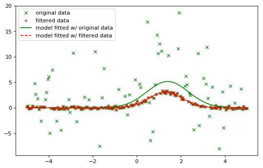
Iterative fitting with sigma clipping:
import numpy as np
from astropy.stats import sigma_clip
from astropy.modeling import models, fitting
import scipy.stats as stats
from matplotlib import pyplot as plt

# Generate fake data with outliers
np.random.seed(0)
x = np.linspace(-5., 5., 200)
y = 3 * np.exp(-0.5 * (x - 1.3)**2 / 0.8**2)
c = stats.bernoulli.rvs(0.35, size=x.shape)
y += (np.random.normal(0., 0.2, x.shape) +
      c*np.random.normal(3.0, 5.0, x.shape))
g_init = models.Gaussian1D(amplitude=1., mean=0, stddev=1.)

# initialize fitters
fit = fitting.LevMarLSQFitter()
or_fit = fitting.FittingWithOutlierRemoval(fit, sigma_clip,
                                           niter=3, sigma=3.0)

# get fitted model and filtered data
or_fitted_model, mask = or_fit(g_init, x, y)
filtered_data = np.ma.masked_array(y, mask=mask)
fitted_model = fit(g_init, x, y)

# plot data and fitted models
plt.figure(figsize=(8,5))
plt.plot(x, y, 'gx', label="original data")
plt.plot(x, filtered_data, 'r+', label="filtered data")
plt.plot(x, fitted_model(x), 'g-',
         label="model fitted w/ original data")
plt.plot(x, or_fitted_model(x), 'r--',
         label="model fitted w/ filtered data")
plt.legend(loc=2, numpoints=1)
()
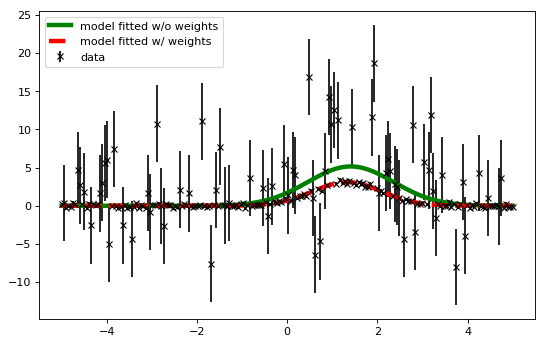
- Fitting with weights from data uncertainties
import numpy as np
from astropy.stats import sigma_clip
from astropy.modeling import models, fitting
import scipy.stats as stats
from matplotlib import pyplot as plt

# Generate fake data with outliers
np.random.seed(0)
x = np.linspace(-5., 5., 200)
y = 3 * np.exp(-0.5 * (x - 1.3)**2 / 0.8**2)
c = stats.bernoulli.rvs(0.35, size=x.shape)
y += (np.random.normal(0., 0.2, x.shape) +
      c*np.random.normal(3.0, 5.0, x.shape))
y_uncs = np.sqrt(np.square(np.full(x.shape, 0.2))
                 + c*np.square(np.full(x.shape,5.0)))
g_init = models.Gaussian1D(amplitude=1., mean=0, stddev=1.)

# initialize fitters
fit = fitting.LevMarLSQFitter()

# fit the data w/o weights
fitted_model = fit(g_init, x, y)

# fit the data using the uncertainties as weights
fitted_model_weights = fit(g_init, x, y, weights=1.0/y_uncs)

# plot data and fitted models
plt.figure(figsize=(8,5))
plt.errorbar(x, y, yerr=y_uncs, fmt='kx', label="data")
plt.plot(x, fitted_model(x), 'g-', linewidth=4.0,
         label="model fitted w/o weights")
plt.plot(x, fitted_model_weights(x), 'r--', linewidth=4.0,
         label="model fitted w/ weights")
plt.legend(loc=2, numpoints=1)
()
Fitters support constrained fitting.
All fitters support fixed (frozen) parameters through the
fixedargument to models or setting thefixedattribute directly on a parameter.For linear fitters, freezing a polynomial coefficient means that the corresponding term will be subtracted from the data before fitting a polynomial without that term to the result. For example, fixing
c0in a polynomial model will fit a polynomial with the zero-th order term missing to the data minus that constant. However, the fixed coefficient value is restored when evaluating the model, to fit the original data values:>>> x = np.arange(1, 10, .1) >>> p1 = models.Polynomial1D(2, c0=[1, 1], c1=[2, 2], c2=[3, 3], ... n_models=2) >>> p1 <Polynomial1D(2, c0=[1., 1.], c1=[2., 2.], c2=[3., 3.], n_models=2)> >>> y = p1(x, model_set_axis=False) >>> p1.c0.fixed = True >>> pfit = fitting.LinearLSQFitter() >>> new_model = pfit(p1, x, y) >>> print(new_model) Model: Polynomial1D Inputs: ('x',) Outputs: ('y',) Model set size: 2 Degree: 2 Parameters: c0 c1 c2 --- --- --- 1.0 2.0 3.0 1.0 2.0 3.0
A parameter can be
tied(linked to another parameter). This can be done in two ways:>>> def tiedfunc(g1): ... mean = 3 * g1.stddev ... return mean >>> g1 = models.Gaussian1D(amplitude=10., mean=3, stddev=.5, ... tied={'mean': tiedfunc})
or:
>>> g1 = models.Gaussian1D(amplitude=10., mean=3, stddev=.5)
>>> g1.mean.tied = tiedfunc
Bounded fitting is supported through the bounds arguments to models or by
setting min and max
attributes on a parameter. Bounds for the
LevMarLSQFitter are always exactly satisfied–if
the value of the parameter is outside the fitting interval, it will be reset to
the value at the bounds. The SLSQPLSQFitter handles
bounds internally.
Different fitters support different types of constraints:
>>> fitting.LinearLSQFitter.supported_constraints
['fixed']
>>> fitting.LevMarLSQFitter.supported_constraints
['fixed', 'tied', 'bounds']
>>> fitting.SLSQPLSQFitter.supported_constraints
['bounds', 'eqcons', 'ineqcons', 'fixed', 'tied']
Note that there are two “constraints” (prior and posterior) that are
not currently used by any of the built-in fitters. They are provided to allow
possible user code that might implement Bayesian fitters (e.g.,
https://gist.github.com/rkiman/5c5e6f80b455851084d112af2f8ed04f).
Plugin Fitters
Fitters defined outside of astropy’s core can be inserted into the
astropy.modeling.fitting namespace through the use of entry points.
Entry points are references to importable objects. A tutorial on
defining entry points can be found in setuptools’ documentation.
Plugin fitters are required to extend from the Fitter
base class. For the fitter to be discovered and inserted into
astropy.modeling.fitting the entry points must be inserted into
the astropy.modeling entry point group
setup(
      # ...
      entry_points = {'astropy.modeling': 'PluginFitterName = fitter_module:PlugFitterClass'}
)
This would allow users to import the PlugFitterName through astropy.modeling.fitting by
from astropy.modeling.fitting import PlugFitterName
One project which uses this functionality is Saba, which insert its SherpaFitter class and thus allows astropy users to use Sherpa’s fitting routine.