Ripley’s K Function Estimators
Spatial correlation functions have been used in the astronomical context to estimate the probability of finding an object, e.g. a galaxy, within a given distance of another object [1].
Ripley’s K function is a type of estimator used to characterize the correlation
of such spatial point processes
[2], [3], [4], [5], [6].
More precisely, it describes correlation among objects in a given field.
The RipleysKEstimator class implements some
estimators for this function which provides several methods for
edge-effects correction.
Basic Usage
The actual implementation of Ripley’s K function estimators lie in the method
evaluate which take the following arguments data, radii, and,
optionally, mode.
The data argument is a 2D array which represents the set of observed
points (events) in the area of study. The radii argument corresponds to a
set of distances for which the estimator will be evaluated. The mode
argument takes a value on the following linguistic set
{none, translation, ohser, var-width, ripley}; each keyword represents a
different method to perform correction due to edge-effects. See the API
documentation and references for details about these methods.
Instances of RipleysKEstimator can also be used as
callables (which is equivalent to calling the evaluate method).
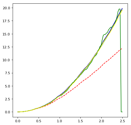
A minimal usage example is shown as follows:
import numpy as np
from matplotlib import pyplot as plt
from astropy.stats import RipleysKEstimator

z = np.random.uniform(low=5, high=10, size=(100, 2))
Kest = RipleysKEstimator(area=25, x_max=10, y_max=10, x_min=5, y_min=5)

r = np.linspace(0, 2.5, 100)
plt.plot(r, Kest.poisson(r), color='green', ls=':', label=r'$K_{pois}$')
plt.plot(r, Kest(data=z, radii=r, mode='none'), color='red', ls='--',
         label=r'$K_{un}$')
plt.plot(r, Kest(data=z, radii=r, mode='translation'), color='black',
         label=r'$K_{trans}$')
plt.plot(r, Kest(data=z, radii=r, mode='ohser'), color='blue', ls='-.',
         label=r'$K_{ohser}$')
plt.plot(r, Kest(data=z, radii=r, mode='var-width'), color='green',
         label=r'$K_{var-width}$')
plt.plot(r, Kest(data=z, radii=r, mode='ripley'), color='yellow',
         label=r'$K_{ripley}$')
()
References
| [1] | Peebles, P.J.E. The large scale structure of the universe. <http://adsabs.harvard.edu/cgi-bin/nph-bib_query?bibcode=1980lssu.book…..P&db_key=AST> |
| [2] | Ripley, B.D. The second-order analysis of stationary point processes. Journal of Applied Probability. 13: 255–266, 1976. |
| [3] | Spatial descriptive statistics. <https://en.wikipedia.org/wiki/Spatial_descriptive_statistics> |
| [4] | Cressie, N.A.C. Statistics for Spatial Data, Wiley, New York. |
| [5] | Stoyan, D., Stoyan, H. Fractals, Random Shapes and Point Fields, Akademie Verlag GmbH, Chichester, 1992. |
| [6] | Correlation function. <https://en.wikipedia.org/wiki/Correlation_function_(astronomy)> |