What’s New in Astropy 3.1?
Overview
Astropy 3.1 is a major release with a focus on performance enhancements, but also adds significant new functionality since the 3.0.x series of releases.
In particular, this release includes:
- Performance Tips
- New Sub-package for Uncertainties and Distributions
- New Box Least Squares Periodogram
- Improvements and New Features in Coordinates
- Improvements and New Features in Table
- Improvements and New Features in Time
- Improvements and New Features in NDData
- New operator for quantities
- Thermodynamic temperature equivalency
- Little-h equivalency
- Change in default cosmology
- Faster Cosmological Calculations
- Improvements in WCSAxes
- New convenience function for imshow with ImageNormalize
- Improvements and New Features in astropy.io.fits
- Common API for World Coordinate Systems
In addition to these major changes, Astropy 3.1 includes a large number of smaller improvements and bug fixes, which are described in the Full Changelog. By the numbers:
- 906 issues have been closed since v3.0
- 437 pull requests have been merged since v3.0
- 92 distinct people have contributed code to this release, 48 of which are first time contributors to Astropy.
Performance Tips
We now include a standard section called Performance tips in the
documentation for each sub-package (when appropriate) which helps you get the
best performance out of a given sub-package. For example, if you want to
improve the performance of your code when using Unit
and Quantity, you can read up about it in the
Performance tips for astropy.units.
New Sub-package for Uncertainties and Distributions
Astropy 3.1 includes a new experimentation sub-package: Uncertainties and Distributions (astropy.uncertainty).
Currently this sub-package provides uncertainty propagation and classes for
representing distributions using a Monte Carlo sampling technique, which is
useful for some cases but certainly not all. The longer-term
plan is to integrate other uncertainty propagation techniques to address typical
astronomy uses cases, including integrating with the already-existing
uncertainty classes that are focused on representing uncertainties in
astropy.nddata.
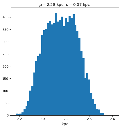
To demonstrate this new functionality, the example below shows propagation of uncertainty in the geometric mean of three numbers that have units:
import numpy as np
from astropy import units as u
from astropy import uncertainty as unc
from astropy.visualization import quantity_support
from matplotlib import pyplot as plt

np.random.seed(12345)

a = unc.normal(1.5*u.kpc, std=50*u.pc, n_samples=10000)
b = unc.uniform(center=3*u.kpc, width=800*u.pc, n_samples=10000)
c = unc.Distribution(((np.random.beta(2,5, 10000)-(2/7))/2 + 3)*u.kpc)
d = (a * b * c) ** (1/3)

with quantity_support():
    plt.hist(d.distribution, bins=50)
    plt.title(r'$\mu={0.value:.2f}$ {0.unit}, $\sigma={1.value:.2f}$ {1.unit}'.format(d.pdf_mean, d.pdf_std))
()
This sub-package should be considered experimental and subject to API changes in the future if user feedback calls for it.
New Box Least Squares Periodogram
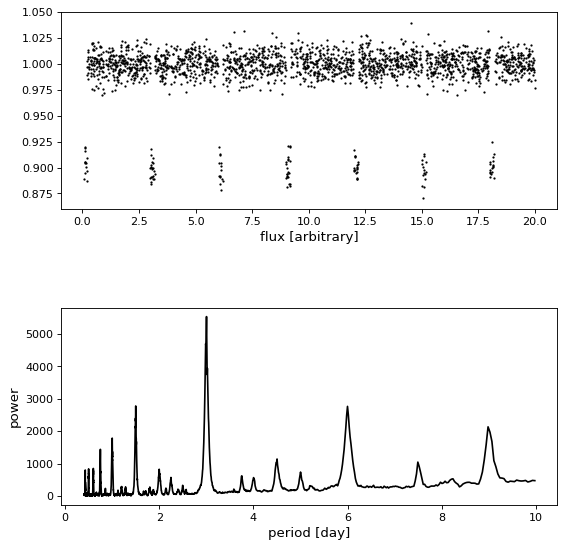
Astropy now has an implementation of the Box least squares (BLS) periodogram
that is commonly used to detect transiting exoplanets and eclipsing
binary star systems. The interface has been designed to match the
LombScargle periodogram, and it can be used with a time series
dataset time, flux, and flux_err as follows:
>>> from astropy import units as u
>>> from astropy.stats import BoxLeastSquares
>>> model = BoxLeastSquares(time * u.day, flux, flux_err=0.01)
>>> duration = 0.2 * u.day
>>> periodogram = model.autopower(duration)
The resulting periodogram will look something like the following when the time series includes a transiting planet:
()
Improvements and New Features in Coordinates
Performance has been improved throughout this sub-package. Highlights include
typically 2-3x faster creation of scalar SkyCoord and
frame classes objects, or up to 20x faster in certain cases. These performance
improvements translate to nearly all convenience methods and operations on
coordinates as well. Coordinate matching is 2-3x faster and can be up to 1000x
faster in certain cases.
A directional_offset_by method has been added
that will yield a new SkyCoord given a “from” coordinate
and an offset:
>>> from astropy import units as u
>>> from astropy.coordinates import SkyCoord
>>> c1 = SkyCoord(1*u.deg, 1*u.deg, frame='icrs')
>>> c1.directional_offset_by(45 * u.deg, 1.414 * u.deg)
<SkyCoord (ICRS): (ra, dec) in deg
  (2.0004075, 1.99964588)>
The from_name method of
SkyCoord now parses “J-coordinate” names (e.g.
“SDSS J153243.67-004342.5”) into their actual coordinate locations. For
example:
>>> from astropy.coordinates import SkyCoord
>>> SkyCoord.from_name('2MASS J06495091-0737408', parse=True)
<SkyCoord (ICRS): (ra, dec) in deg
  (102.462125, -7.628)>
Additionally, the of_address convenience
method now gets coordinates from OpenStreetMap. Google Maps is still supported
but only if you provide your own API key (due to Google new requiring a key) -
see of_address for more details.
Improvements and New Features in Table
The Table class now supports fine-grained control of the way to
write out (serialize) the columns in a Table to FITS, HDF5, ECSV, or YAML. In
particular one can specify on a per-class or per-column basis how to write
Time and masked columns. For details see Table serialization
methods.
A new table index engine SCEngine was added which uses the Sorted
Containers package. This provides
the capability for efficiently maintaining an indexed table when the table is
being modified (for instance adding new rows). It replaces the deprecated
FastRBT engine as the preferred engine in this case.
Support for use of Time and TimeDelta columns
within a Table was improved significantly:
Improvements and New Features in Time
Array-valued Time and TimeDelta objects are now
“mutable” and one can set items or slices like normal arrays. In general the
the right-side set value will be converted as needed to match attributes like
time scale of the object. For details see Get and set values.
New strftime and strptime methods were
added to the Time class. These methods are similar to those in
the Python standard library time package and provide flexible input and output
formatting. However, the astropy versions also include fractional second
support.
A new datetime64 format was added to the Time class to
support working with numpy.datetime64 dtype arrays.
A potentially important API change to note is removing timescale from the string
version of FITS format time string. Previous versions of astropy incorrectly
included the time scale as part of the string (e.g.
2010-01-01T00:00:34.000(TAI)). However, the timescale is not part of the
FITS standard and should not be included, so this has been fixed. For now
strings in this format will be parsed, but this behavior is deprecated and
should no longer be relied on. New FITS strings produced by the
Time object will no longer include the scale, in line with the
standard.
Improvements and New Features in NDData
New uncertainty types
Two new uncertainty types, VarianceUncertainty and
InverseVariance, have been added for use with the gridded
data types in NDData. As with StdDevUncertainty, these
uncertainties are propagated when used with CCDData.
Support for working with bit planes and converting them to binary masks
A new function for converting bit planes to binary masks,
bitfield_to_boolean_mask, supports a very flexible way to
specify which planes to include in calculating masks. See
Utility functions for handling bit masks and mask arrays. for details and several examples.
Improvements and New Features for Units and Quantities
New operator for quantities
The easiest way to create a Quantity until now has been to
multiply scalars or arrays by units, for example:
>>> import numpy as np
>>> from astropy import units as u
>>> array = np.arange(1000000)
>>> quantity = array * u.m / u.s
However, this can be inefficient, because the array is copied, and in addition
to using up more memory, this makes things slow. We have now introduced a new
operator that creates a Quantity without copying the data:
>>> quantity = array << u.m / u.s
Depending on the size of the array, this can be several times faster than using
the * operator. Note that this means that the quantity and the array now
share the same memory (so modifying the array will modify the quantity).
Thermodynamic temperature equivalency
The new thermodynamic_temperature() cosmology
equivalency allows conversion between Jy/beam and “thermodynamic temperature”,
\(T_{CMB}\), in Kelvins. For example:
>>> import astropy.units as u
>>> nu = 143 * u.GHz
>>> t_k = 0.002632051878 * u.K
>>> t_k.to(u.MJy / u.sr, equivalencies=u.thermodynamic_temperature(nu))
<Quantity 1. MJy / sr>
See Thermodynamic Temperature Equivalency for more details.
Little-h equivalency
The new with_H0() equivalency allows
conversion between physical units and so called “little-h” units, a frequent
source of confusion for novice (and not-so-novice…) extragalactic astronomers
and cosmologists. To see it in action:
>>> import astropy.units as u
>>> from astropy.cosmology import WMAP9
>>> distance = 70 * (u.Mpc/u.littleh)
>>> distance
<Quantity 70. Mpc / littleh>
>>> distance.to(u.Mpc, u.with_H0(WMAP9.H0))
<Quantity 100.98095788 Mpc>
See Reduced Hubble constant/”little-h” Equivalency for more details.
Improvements for Cosmology
Change in default cosmology
The default cosmology returned by the astropy.cosmology.default_cosmology
configuration item has been changed from the WMAP 9 year results to the Planck
2015 results - as a result, you may see small changes in results of calculations
where the cosmology was not explicitly specified. The default cosmology
infrastructure is only provided for convenience and should be expected to
change over time - as a result, for reproducibility it is always best to use
an explicit cosmology rather than rely on the default.
Faster Cosmological Calculations
There are now significant speedups (up to 100x) for distance and age calculations for FlatLambdaCDM cosmologies with no radiation or neutrinos, including de Sitter and Einstein-de Sitter cosmologies. For example, calculations such as:
>> import astropy.units as u
>> from astropy.cosmology import FlatLambdaCDM
>> FlatLambdaCDM(H0=60 * u.km / u.sec / u.Mpc, Om0=0.3, Tcmb0=0)
>> cosmology.age([1.0, 2.0, 3.0])
will now be significantly faster.
Improvements and New Features in astropy.visualization
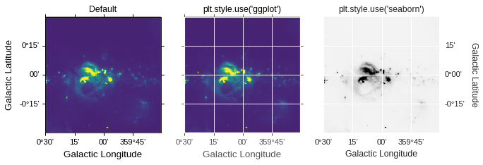
Improvements in WCSAxes
The WCSAxes framework for making plots of astronomical images with Matplotlib
has been improved in this release - in particular, Matplotlib styles (e.g.
plt.style.use('ggplot')) and
rcParams should now be
correctly taken into account, and the default spacing of tick labels from the
ticks should now be improved. The following shows an example of using the
default, the ggplot, and the seaborn styles:
()
By default, Right Ascension coordinates will now default to being formatted in
hours rather than in degrees. Finally, there have been a number of
improvements to the API, including for example the ability to use the Matplotlib
tick_params
method, the ability to more easily set the
tick labels to be decimal using the decimal=True option to
set_format_unit(), and
the ability to control whether the ticks should be facing inwards or outwards using
the direction='in'/'out' argument to set_ticks().
In addition to these improvements, drawing of contours has now been made significantly faster, by factors of 10-100x depending on the specific contours shown.
New convenience function for imshow with ImageNormalize
A new imshow_norm function has been created to simplify
the display of images using matplotlib with astronomy-appropriate stretches.
Specifically, it allows plotting an image using matplotlib’s imshow, using the
visualization stretch and interval classes, but all in a single
compact function call:
import matplotlib.pyplot as plt
from astropy.utils.data import get_pkg_data_filename
from astropy.io import fits
from astropy.visualization import imshow_norm, PercentileInterval, SqrtStretch

# Get an example dataset
img_fn = get_pkg_data_filename('visualization/reprojected_sdss_r.fits.bz2')
image = fits.getdata(img_fn, 0)

# plot the central 99th percentile with a sqrt stretch in one call
imshow_norm(image, origin='lower',
            interval=PercentileInterval(99), stretch=SqrtStretch())
plt.colorbar(orientation='horizontal')
()
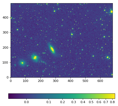
See the Image stretching and normalization section for more details on this and related features.
Improvements and New Features in astropy.io.fits
The fitsheader command line tool now supports a dfits+fitsort mode,
and the dotted notation for keywords (e.g. ESO.INS.ID):
$ fitsheader --fitsort astropy/io/fits/tests/data/test* -k DATE-OBS -k ORIGIN
               filename               DATE-OBS                 ORIGIN
------------------------------------- -------- --------------------------------------
astropy/io/fits/tests/data/test0.fits 19/05/94 NOAO-IRAF FITS Image Kernel Aug 1 1997
astropy/io/fits/tests/data/test1.fits 19/05/94 NOAO-IRAF FITS Image Kernel Aug 1 1997
Common API for World Coordinate Systems
We have designed a new general programmatic interface for objects that represent
world coordinate system (WCS) transformations, and astropy’s own
WCS now implements this interface. One of the highlights
of this interface is the ability to transform to/from astropy objects such as
SkyCoord or Quantity
objects:
>>> from astropy.wcs import WCS
>>> from astropy.coordinates import SkyCoord
>>> from astropy.utils.data import get_pkg_data_filename
>>> from astropy.io import fits
>>> filename = get_pkg_data_filename('galactic_center/gc_2mass_k.fits')
>>> wcs = WCS(filename)
>>> wcs.pixel_to_world([1, 2], [4, 3])
<SkyCoord (FK5: equinox=2000.0): (ra, dec) in deg
    [(266.97242993, -29.42584415), (266.97084321, -29.42723968)]>
>>> wcs.world_to_pixel(SkyCoord('00h00m00s +00d00m00s', frame='galactic'))
[array(356.85179997), array(357.45340331)]
You can find out more about using this new API in Shared Python interface for World Coordinate Systems.
For anyone interested in implementing this interface in other WCS classes, we recommend reading the Astropy Proposal for Enhancement 14: A shared Python interface for World Coordinate Systems (APE 14), and we have provided base classes defining the API, as well as wrapper classes to help automatically implement the high-level class.
Full change log
To see a detailed list of all changes in version v3.1, including changes in API, please see the Full Changelog.
Contributors to the v3.1 release
|
|
|
|
Where a * indicates their first contribution to Astropy.