Efficient Model Rendering with Bounding Boxes

New in version 1.1.

All Model subclasses have a bounding_box attribute that can be used to set the limits over which the model is significant. This greatly improves the efficiency of evaluation when the input range is much larger than the characteristic width of the model itself. For example, to create a sky model image from a large survey catalog, each source should only be evaluated over the pixels to which it contributes a significant amount of flux. This task can otherwise be computationally prohibitive on an average CPU.

The Model.render method can be used to evaluate a model on an output array, or input coordinate arrays, limiting the evaluation to the bounding_box region if it is set. This function will also produce postage stamp images of the model if no other input array is passed. To instead extract postage stamps from the data array itself, see 2D Cutout Images.

Using the Bounding Box

For basic usage, see Model.bounding_box. By default no bounding_box is set, except on model subclasses where a bounding_box property or method is explicitly defined. The default is then the minimum rectangular region symmetric about the position that fully contains the model. If the model does not have a finite extent, the containment criteria are noted in the documentation. For example, see Gaussian2D.bounding_box.

Model.bounding_box can be set by the user to any callable. This is particularly useful for fitting models created with custom_model or as a compound model:

>>> from astropy.modeling import custom_model
>>> def ellipsoid(x, y, z, x0=0, y0=0, z0=0, a=2, b=3, c=4, amp=1):
...     rsq = ((x - x0) / a) ** 2 + ((y - y0) / b) ** 2 + ((z - z0) / c) ** 2
...     val = (rsq < 1) * amp
...     return val
...
>>> class Ellipsoid3D(custom_model(ellipsoid)):
...     # A 3D ellipsoid model
...     @property
...     def bounding_box(self):
...         return ((self.z0 - self.c, self.z0 + self.c),
...                 (self.y0 - self.b, self.y0 + self.b),
...                 (self.x0 - self.a, self.x0 + self.a))
...
>>> model = Ellipsoid3D()
>>> model.bounding_box
((-4.0, 4.0), (-3.0, 3.0), (-2.0, 2.0))

Warning

Currently when creating a new compound model by combining multiple models, the bounding boxes of the components (if any) are not currently combined. So bounding boxes for compound models must be assigned explicitly. A future release will determine the appropriate bounding box for a compound model where possible.

Efficient evaluation with Model.render()

When a model is evaluated over a range much larger than the model itself, it may be prudent to use the Model.render method if efficiency is a concern. The render method can be used to evaluate the model on an array of the same dimensions. model.render() can be called with no arguments to return a “postage stamp” of the bounding box region.

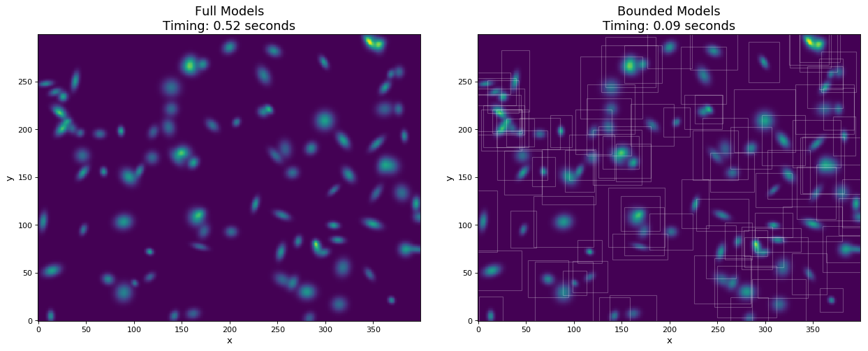
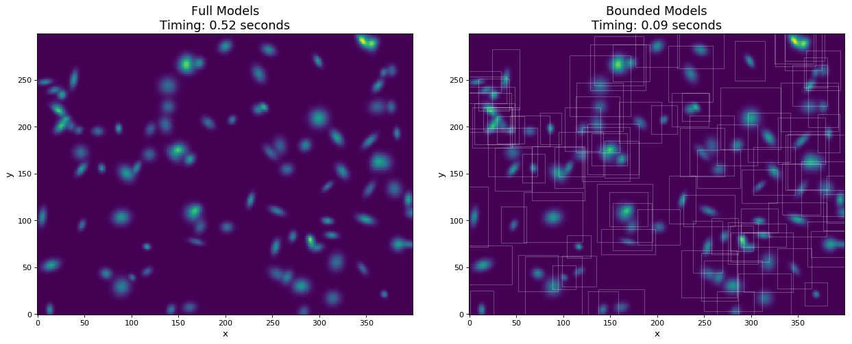
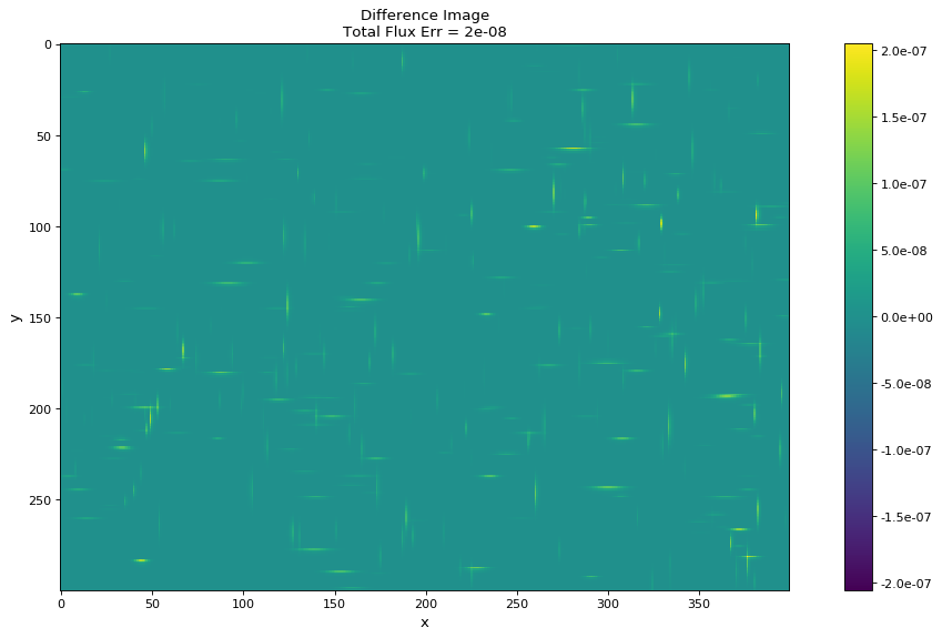
In this example, we generate a 300x400 pixel image of 100 2D Gaussian sources. For comparison, the models are evaluated both with and without using bounding boxes. By using bounding boxes, the evaluation speed increases by approximately a factor of 10 with negligible loss of information.

import numpy as np
from time import time
from astropy.modeling import models
import matplotlib.pyplot as plt
from matplotlib.patches import Rectangle

imshape = (300, 400)
y, x = np.indices(imshape)

# Generate random source model list
np.random.seed(0)
nsrc = 100
model_params = [
    dict(amplitude=np.random.uniform(.5, 1),
         x_mean=np.random.uniform(0, imshape[1] - 1),
         y_mean=np.random.uniform(0, imshape[0] - 1),
         x_stddev=np.random.uniform(2, 6),
         y_stddev=np.random.uniform(2, 6),
         theta=np.random.uniform(0, 2 * np.pi))
    for _ in range(nsrc)]

model_list = [models.Gaussian2D(**kwargs) for kwargs in model_params]

# Render models to image using bounding boxes
bb_image = np.zeros(imshape)
t_bb = time()
for model in model_list:
    model.render(bb_image)
t_bb = time() - t_bb

# Render models to image using full evaluation
full_image = np.zeros(imshape)
t_full = time()
for model in model_list:
    model.bounding_box = None
    model.render(full_image)
t_full = time() - t_full

flux = full_image.sum()
diff = (full_image - bb_image)
max_err = diff.max()

# Plots
plt.figure(figsize=(16, 7))
plt.subplots_adjust(left=.05, right=.97, bottom=.03, top=.97, wspace=0.15)

# Full model image
plt.subplot(121)
plt.imshow(full_image, origin='lower')
plt.title('Full Models\nTiming: {:.2f} seconds'.format(t_full), fontsize=16)
plt.xlabel('x')
plt.ylabel('y')

# Bounded model image with boxes overplotted
ax = plt.subplot(122)
plt.imshow(bb_image, origin='lower')
for model in model_list:
    del model.bounding_box  # Reset bounding_box to its default
    dy, dx = np.diff(model.bounding_box).flatten()
    pos = (model.x_mean.value - dx / 2, model.y_mean.value - dy / 2)
    r = Rectangle(pos, dx, dy, edgecolor='w', facecolor='none', alpha=.25)
    ax.add_patch(r)
plt.title('Bounded Models\nTiming: {:.2f} seconds'.format(t_bb), fontsize=16)
plt.xlabel('x')
plt.ylabel('y')

# Difference image
plt.figure(figsize=(16, 8))
plt.subplot(111)
plt.imshow(diff, vmin=-max_err, vmax=max_err)
plt.colorbar(format='%.1e')
plt.title('Difference Image\nTotal Flux Err = {:.0e}'.format(
    ((flux - np.sum(bb_image)) / flux)))
plt.xlabel('x')
plt.ylabel('y')
plt.show()

(png, svg, pdf)

(png, svg, pdf)