Instantiating and Evaluating Models
The base class of all models is Model, however
fittable models should subclass FittableModel.
Fittable models can be linear or nonlinear in a regression analysis sense.
In general models are instantiated by providing the parameter values that define that instance of the model to the constructor, as demonstrated in the section on Parameters.
Additionally, a Model instance may represent a single model
with one set of parameters, or a model set consisting of a set of parameters
each representing a different parameterization of the same parametric model.
For example one may instantiate a single Gaussian model with one mean, standard
deviation, and amplitude. Or one may create a set of N Gaussians, each one of
which would be fitted to, for example, a different plane in an image cube.
Regardless of whether using a single model, or a model set, parameter values may be scalar values, or arrays of any size and shape, so long as they are compatible according to the standard Numpy broadcasting rules. For example, a model may be instantiated with all scalar parameters:
>>> from astropy.modeling.models import Gaussian1D
>>> g = Gaussian1D(amplitude=1, mean=0, stddev=1)
>>> g
<Gaussian1D(amplitude=1., mean=0., stddev=1.)>
The newly created model instance g now works like a Gaussian function
with the given parameters fixed. It takes a single input:
>>> g.inputs
('x',)
>>> g(x=0)
1.0
The model can also be called without explicitly using keyword arguments:
>>> g(0)
1.0
Or it may use all array parameters. For example if all parameters are 2x2 arrays the model is computed element-wise using all elements in the arrays:
>>> g = Gaussian1D(amplitude=[[1, 2], [3, 4]], mean=[[0, 1], [1, 0]],
...                stddev=[[0.1, 0.2], [0.3, 0.4]])
>>> g
<Gaussian1D(amplitude=[[1., 2.], [3., 4.]], mean=[[0., 1.], [1., 0.]],
stddev=[[0.1, 0.2], [0.3, 0.4]])>
>>> g(0)
array([[1.00000000e+00, 7.45330634e-06],
       [1.15977604e-02, 4.00000000e+00]])
Or it may even use a mix of scalar values and arrays of different sizes and dimensions so long as they are compatible:
>>> g = Gaussian1D(amplitude=[[1, 2], [3, 4]], mean=0.1, stddev=[0.1, 0.2])
>>> g(0)
array([[0.60653066, 1.76499381],
       [1.81959198, 3.52998761]])
In this case, four values are computed–one using each element of the amplitude array. Each model uses a mean of 0.1, and a standard deviation of 0.1 is used with the amplitudes of 1 and 3, and 0.2 is used with amplitudes 2 and 4.
If any of the parameters have incompatible values this will result in an error:
>>> g = Gaussian1D(amplitude=1, mean=[1, 2], stddev=[1, 2, 3])
Traceback (most recent call last):
...
InputParameterError: Parameter 'mean' of shape (2,) cannot be broadcast
with parameter 'stddev' of shape (3,).  All parameter arrays must have
shapes that are mutually compatible according to the broadcasting rules.
Model Sets
By default, Model instances represent a single model.
There are two ways, when instantiating a Model instance, to
create a model set instead. The first is to specify the n_models argument
when instantiating the model:
>>> g = Gaussian1D(amplitude=[1, 2], mean=[0, 0], stddev=[0.1, 0.2],
...                n_models=2)
>>> g
<Gaussian1D(amplitude=[1., 2.], mean=[0., 0.], stddev=[0.1, 0.2],
n_models=2)>
When specifying some n_models=N this requires that the parameter values be
arrays of some kind, the first axis of which has as length of N. This
axis is referred to as the model_set_axis, and by default is is the 0th
axis of parameter arrays. In this case the parameters were given as 1-D arrays
of length 2. The values amplitude=1, mean=0, stddev=0.1 are the parameters
for the first model in the set. The values amplitude=2, mean=0, stddev=0.2
are the parameters defining the second model in the set.
This has different semantics from simply using array values for the parameters, in that ensures that parameter values and input values are matched up according to the model_set_axis before any other array broadcasting rules are applied.
For example, in the previous section we created a model with array values like:
>>> g = Gaussian1D(amplitude=[[1, 2], [3, 4]], mean=0.1, stddev=[0.1, 0.2])
If instead we treat the rows as values for two different model sets, this particular instantiation will fail, since only one value is given for mean:
>>> g = Gaussian1D(amplitude=[[1, 2], [3, 4]], mean=0.1, stddev=[0.1, 0.2],
...                n_models=2)
Traceback (most recent call last):
...
InputParameterError: All parameter values must be arrays of dimension at
least 1 for model_set_axis=0 (the value given for 'mean' is only
0-dimensional)
To get around this for now, provide two values for mean:
>>> g = Gaussian1D(amplitude=[[1, 2], [3, 4]], mean=[0.1, 0.1],
...                stddev=[0.1, 0.2], n_models=2)
This is different from the case without n_models=2. It does not mean that
the value of amplitude is a 2x2 array. Rather, it means there are two values
for amplitude (one for each model in the set), each of which is 1-D array of
length 2. The value for the first model is [1, 2], and the value for the
second model is [3, 4]. Likewise, scalar values are given for the mean and
standard deviation of each model in the set.
When evaluating this model on a single input we get a different result from the single-model case:
>>> g(0)
array([[0.60653066, 1.21306132],
       [2.64749071, 3.52998761]])
Each row in this output is the output for each model in the set. The first is
the value of the Gaussian with amplitude=[1, 2], mean=0.1, stddev=0.1, and
the second is the value of the Gaussian with amplitude=[3, 4], mean=0.1,
stddev=0.2.
We can also pass a different input to each model in a model set by passing in an array input:
>>> g([0, 1])
array([[6.06530660e-01, 1.21306132e+00],
       [1.20195892e-04, 1.60261190e-04]])
By default this uses the same concept of a model_set_axis. The first
dimension of the input array is used to map inputs to corresponding models in
the model set. We can use this, for example, to evaluate the model on 1-D
array inputs with a different input to each model set:
>>> g([[0, 1], [2, 3]])
array([[6.06530660e-01, 5.15351422e-18],
       [7.57849134e-20, 8.84815213e-46]])
In this case the first model is evaluated on [0, 1], and the second model
is evaluated on [2, 3]. If the input has length greater than the number of
models in the set then this is in error:
>>> g([0, 1, 2])
Traceback (most recent call last):
...
ValueError: Input argument 'x' does not have the correct dimensions in
model_set_axis=0 for a model set with n_models=2.
And input like [0, 1, 2] wouldn’t work anyways because it is not compatible
with the array dimensions of the parameter values. However, what if we wanted
to evaluate all models in the set on the input [0, 1]? We could do this
by simply repeating:
>>> g([[0, 1], [0, 1]])
array([[6.06530660e-01, 5.15351422e-18],
       [2.64749071e+00, 1.60261190e-04]])
But there is a workaround for this use case that does not necessitate
duplication. This is to include the argument model_set_axis=False:
>>> g([0, 1], model_set_axis=False)
array([[6.06530660e-01, 5.15351422e-18],
       [2.64749071e+00, 1.60261190e-04]])
What model_set_axis=False implies is that an array-like input should not be
treated as though any of its dimensions map to models in a model set. And
rather, the given input should be used to evaluate all the models in the model
set. For scalar inputs like g(0), model_set_axis=False is implied
automatically. But for array inputs it is necessary to avoid ambiguity.
Model Inverses
All models have a Model.inverse property
which may, for some models, return a new model that is the analytic inverse of
the model it is attached to. For example:
>>> from astropy.modeling.models import Linear1D
>>> linear = Linear1D(slope=0.8, intercept=1.0)
>>> linear.inverse
<Linear1D(slope=1.25, intercept=-1.25)>
The inverse of a model will always be a fully instantiated model in its own right, and so can be evaluated directly like:
>>> linear.inverse(2.0)
1.25
It is also possible to assign a custom inverse to a model. This may be useful, for example, in cases where a model does not have an analytic inverse, but may have an approximate inverse that was computed numerically and is represented by a polynomial. This works even if the target model has a default analytic inverse–in this case the default is overridden with the custom inverse:
>>> from astropy.modeling.models import Polynomial1D
>>> linear.inverse = Polynomial1D(degree=1, c0=-1.25, c1=1.25)
>>> linear.inverse
<Polynomial1D(1, c0=-1.25, c1=1.25)>
If a custom inverse has been assigned to a model, it can be deleted with
del model.inverse. This resets the inverse to its default (if one exists).
If a default does not exist, accessing model.inverse raises a
NotImplementedError. For example polynomial models do not have a default
inverse:
>>> del linear.inverse
>>> linear.inverse
<Linear1D(slope=1.25, intercept=-1.25)>
>>> p = Polynomial1D(degree=2, c0=1.0, c1=2.0, c2=3.0)
>>> p.inverse
Traceback (most recent call last):
  File "<stdin>", line 1, in <module>
  File "astropy\modeling\core.py", line 796, in inverse
    raise NotImplementedError("An analytical inverse transform has not "
NotImplementedError: An analytical inverse transform has not been
implemented for this model.
One may certainly compute an inverse and assign it to a polynomial model though.
Note
When assigning a custom inverse to a model no validation is performed to ensure that it is actually an inverse or even approximate inverse. So assign custom inverses at your own risk.
Model Separability
Simple models have a boolean Model.separable property.
It indicates whether the outputs are independent and is essential for computing the
separability of compound models using the is_separable() function.
Having a separable compound model means that it can be decomposed into independent models,
which in turn is useful in many applications.
For example, it may be easier to define inverses using the independent parts of a model
than the entire model.
In other cases, tools using GWCS,
can be more flexible and take advantage of separable spectral and spatial transforms.
Further examples
The examples here assume this import statement was executed:
>>> from astropy.modeling.models import Gaussian1D, Polynomial1D
>>> import numpy as np
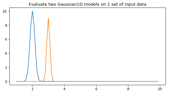
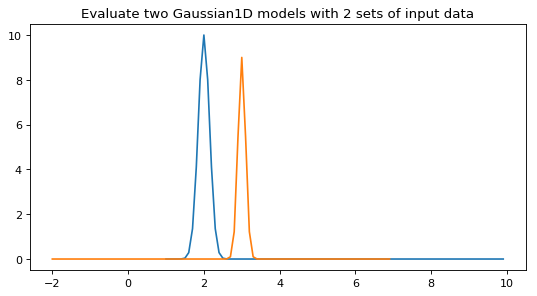
Create a model set of two 1-D Gaussians:
>>> x = np.arange(1, 10, .1)
>>> g1 = Gaussian1D(amplitude=[10, 9], mean=[2, 3],
...                 stddev=[0.15, .1], n_models=2)
>>> print(g1)
Model: Gaussian1D
Inputs: ('x',)
Outputs: ('y',)
Model set size: 2
Parameters:
    amplitude mean stddev
    --------- ---- ------
         10.0  2.0   0.15
          9.0  3.0    0.1
Evaluate all models in the set on one set of input coordinates:
>>> y = g1(x, model_set_axis=False)  # broadcast the array to all models
>>> y.shape
(2, 90)
or different inputs for each model in the set:
>>> y = g1([x, x + 3])
>>> y.shape
(2, 90)
()
()
Evaluating a set of multiple polynomial models with one input data set creates multiple output data sets:
>>> p1 = Polynomial1D(degree=1, n_models=5)
>>> p1.c1 = [0, 1, 2, 3, 4]
>>> print(p1)
Model: Polynomial1D
Inputs: ('x',)
Outputs: ('y',)
Model set size: 5
Degree: 1
Parameters:
     c0  c1
    --- ---
    0.0 0.0
    0.0 1.0
    0.0 2.0
    0.0 3.0
    0.0 4.0
>>> y = p1(x, model_set_axis=False)
()
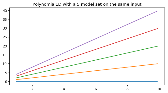
When passed a 2-D array, the same polynomial will map each row of the array to one model in the set, one for one:
>>> x = np.arange(30).reshape(5, 6)
>>> y = p1(x)
>>> y
array([[  0.,   0.,   0.,   0.,   0.,   0.],
       [  6.,   7.,   8.,   9.,  10.,  11.],
       [ 24.,  26.,  28.,  30.,  32.,  34.],
       [ 54.,  57.,  60.,  63.,  66.,  69.],
       [ 96., 100., 104., 108., 112., 116.]])
>>> y.shape
(5, 6)